Models, Sources, and Seeds in dbt: A Complete Tutorial for Transforming Data with Reproducible SQL

Welcome to the second part of this series on DBT. In the first installment, we did a general introduction to this data transformation framework, covered its core concepts, the components of a project, and ran a set of simple commands to initialize our first data transformation process. If you missed it, you can read it here.

We’ll dive deeper into several of the concepts already mentioned, focusing on understanding them thoroughly and taking full advantage of the tool’s capabilities. We’ll cover models, data sources, and seeds, and keep professionalizing our test project.

Models

This is the heart of our project. In DBT, a model is simply a SQL file containing a SELECT statement, nothing more, nothing less. While that sounds pretty straightforward, behind the scenes models function as abstractions that let us create modular, maintainable, version-controlled, and testable transformation logic for our data warehouse. Let’s take a closer look at what they are and how they work.

What Is a Model, Really?

A model is a .sql file located in the models/ directory of our DBT project. Each model typically represents a transformation step, such as data cleaning, setting a column’s type, aggregating or summarizing data, joining data sources, or countless other options. Let’s look at a simple model example:

In this case, we’re selecting active customers and referencing the raw_customers model using the ref() function (which we’ll explore in more depth shortly) to indicate where the data comes from. Here, we can reference raw data sources like data warehouses or we can point to another model’s output. That’s how transformations get chained together. My reference to raw_customers could just as easily have been to a hypothetical int_select_customers, a previous .sql file that filters the customers we want to work with.

When we use the dbt run command to execute our models, they get compiled into SQL and run against our data warehouse, resulting in a materialization usually in the form of a view or table (DBT supports other materialization types but they’re much less common), depending on how we configure it. In fact, once executed we can inspect the compiled code in the target/compiled directory and see how abstractions like ref() translate into raw SQL.

Now, let’s analyze the parts of a model.

SQL Logic

As mentioned earlier, the SELECT statement is the core of the model. It can be as simple or as complex as needed, with filters, joins, subqueries, CTEs… We have the full SQL arsenal at our disposal.

The ref() Function

This function is used to reference another model and serves several roles:

• It tells DBT there’s a dependency between models.
• It resolves to the correct schema or table at execution time.
• It helps DBT build a DAG (which stands for “directed acyclic graph”) of model dependencies.

When in our example we use FROM {{ ref(‘raw_customers’) }}, DBT understands that it must first build ‘raw_customers’ before executing our current model.

Model Configurations and Settings

Models in DBT can have specific configurations that determine how and where results are materialized, how resulting tables are named, or how they’re grouped for automated tasks, among other things. These configurations are defined at the top of the model’s .sql file using the {{ config(…) }} block or in the dbt_project.yml file.

Let’s look at the most common parameters and their uses:

materialized

This is probably the most important setting, as it defines how the model’s result is materialized in the data warehouse. It can take one of the following values:

• view: the model’s result is created as a view and is the default option. It doesn’t take up disk space and always reflects up-to-date data, though it may imply higher compute costs when queried.
• table: the model materializes as a table. This means data is persisted at dbt run time. It’s ideal for heavy transformations or when query time optimization is needed.
• incremental: this option allows updating only part of the data each time the model runs, rather than recreating the entire table. It’s useful for handling large data volumes in production pipelines.
• ephemeral: not materialized in the warehouse. The model becomes a CTE (Common Table Expression) within another model that consumes it. It’s the best option for intermediate steps that you don’t want to persist.

schema

Allows overriding the default schema configured in the project. Useful when you want to segment your models by environment (e.g., dev, staging, prod) or by specific processes.

alias

Controls the final name under which the table or view is created in the warehouse. By default, DBT uses the .sql filename as the generated table name, but with alias you can change it while maintaining file naming conventions in your transformation process.

tags

Allow labeling models for logical grouping. These tags can then be used to run only a specific part of the project with commands like dbt run –select tag:incrementals, or for analysis and documentation purposes.

Sources

In every DBT model, the first step is consuming data that already exists in our system: transactional databases, third-party systems, APIs, or any source we deem necessary or appropriate. Within the DBT framework, these external sources (i.e., tables not generated by DBT but already present in the data warehouse) are configured as sources.

This lets DBT know that those data are part of our transformation logic and enables us to use features like automatic tests, centralized documentation, and clear visualization in the dependency DAG.

Defining Sources

Data sources are defined in .yml files within the models/ directory, typically in files like src_*.yml, though no specific naming convention is required; any name works. There we use a YAML structure to register our external data.

In this case, we have the following components:

• raw_db is a logical identifier for the source database.
• schema defines the warehouse schema where the actual tables live.
• tables is the list of concrete tables we want to use as sources.

Implementing Sources

Now that we have the data sources defined in our YAML and ready to use… how do we actually implement them in our model? That’s where the source() function comes in. Let’s look at a small example:

In these two simple lines of code, we’re telling DBT: “I want to consume the customers table in the raw schema that’s part of the rawdb source.” In other words, just like with the _ref() function, DBT abstracts much of the behind-the-scenes work through functions. But unlike ref(), source() is used to reference external data.

Using source() also provides several benefits over directly using the table name in the model:

• Traceability and documentation: DBT can include this data in the automatically generated documentation using the dbt docs generate command (which we’ll use later to create our project’s documentation).
• Tests: We can apply automatic tests on external tables (like verifying they don’t have null values, that they have a valid primary key, among many other options).
• Change management: If the schema or table name changes, we only need to modify it in the .yml file and not in every model.
• DAG visualization: Sources appear as nodes in the dependency graph, making it much easier to understand the complete flow.

Additional Configurations

The last thing we’ll cover about sources today are two simple but useful additional configurations for defining our sources. For example, we can document both sources and tables:

And we can declare tests we want to implement on our source tables:

This ensures that customer_id is unique and not null. Defining solid tests is an excellent practice for making our data transformation pipelines robust.

Seeds

The last component we’ll cover today is seeds. In DBT, seeds are CSV files that live within the project and get loaded directly into the data warehouse as tables. They function as small static databases: they can represent reference catalogs, code lists, business rules, mappings, or even test data. In other words, they’re especially useful when we have a dataset that won’t change or will only change in very controlled ways, like a company’s list of operating countries or a small list of suppliers.

This capability is especially useful when we want to incorporate simple or team-controlled datasets without depending on external integrations or complex ingestion processes. We copy the CSV into the /seeds folder in our directory, run the dbt seed command, and we’re ready to consume that data.

The key difference between seeds and sources when using the data is that seeds are referenced with the ref() function we’ve already seen, just like models. We’ll see a seed in action in the demo.

Demo Time!

Now that we have these concepts well baked, let’s keep moving forward with the demo we started in the last post. First things first, to keep the project organized, let’s delete the my_project/models/example folder that DBT auto-generated when initializing the project, and then we’ll create a dummy database so we have some data to process and see results.

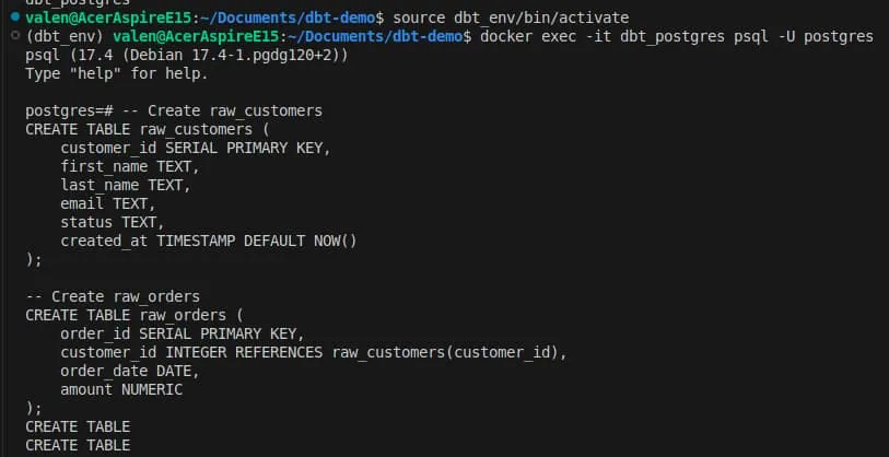
To spin up the Docker container again (unless you’ve patiently waited all these weeks with your computer on and the container running), let’s run these commands in our terminal to activate the virtual environment we created last time and start the container:

Starting the dbt_postgres container and connecting with psql inside the dbt virtual environment

Now, let’s create two dummy tables inside our container so we can build some transformations in DBT. Copy and paste the following code in the terminal.

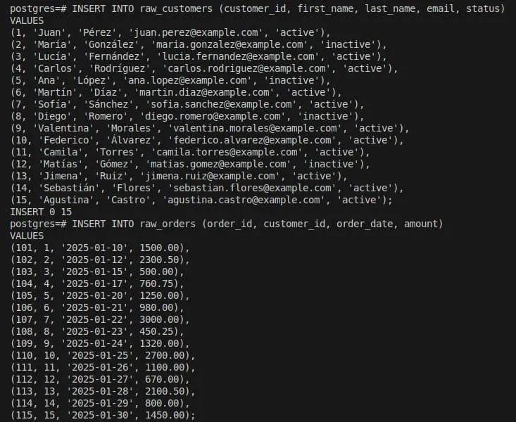
Now let’s add dummy data. Here’s the raw_customers data:

And here’s the raw_orders data:

Then you can run this query to verify the contents of the tables we created:

Now let’s define and configure our new sources. Inside the models folder (my_project/models/), we’ll create a YAML file called src_raw_data.yml. In it, we’ll paste the following content:

We now have both tables defined as sources in our project, and we’ve also configured a couple of tests (uniqueness and non-nullability of the IDs). Next step, let’s update our dbt_project.yml file to include the new model information. Put this code in:

Here we’ve set the configurations for our models in the project’s general file and defined our materialization strategy as “view.” Now we can finally create our intermediate model! Inside the /models folder, let’s create a new .sql file and paste the following SQL code.

This is a model just like the one we saw at the beginning of the post. What it does is take our two sources, assign them an alias, and join them using our customer_id. Now, to run it, execute the following command:

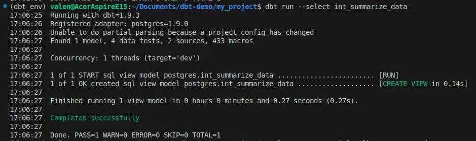
dbt run –select int_summarize_data

If you did everything correctly, you should see something like this:

If you want to see the compiled code, you can run this:

dbt compile –select int_summarize_data

And if we want to see the result of what was materialized as a view, we can do it with this line:

psql -U postgres -h localhost -p 5432 -d postgres -c “SELECT * FROM postgres.int_summarize_data LIMIT 10;”

This will ask for the password we defined last time in the profiles.yml file. The result should be:

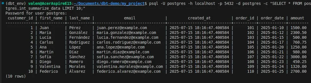
Done! We’ve now run our first custom DBT model and joined data from both tables using customer_id as the common key. We can now see the first name, last name, email, creation date, order number, order date, and order amount for each of our customers.

To close out today’s demo, we’ll create a seed and use it to classify our sales by size. You can find the CSV with the data here and download it directly (delete the “- Hoja 1” from the name!). This file contains order classification categories for our customers, and since it’s static, brief data that won’t change frequently, it’s appropriate to treat it as a seed.

If you look, beneath the /models folder we have one called seeds. We’ll place our freshly downloaded file there and update our dbt_project.yml with the seed configuration.

With all that done, we can run the seed to load it.

dbt seed

The result should look something like this:

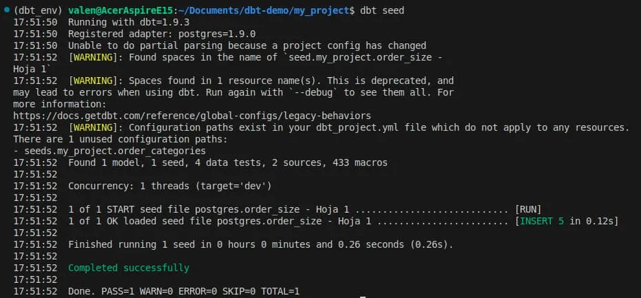
After that, we’ll create a new intermediate. We’ll call it int_categorize_orders and it’ll be a .sql file. In it, we’ll put the following query.

Now, if we run this model, we’ll unify our transformations.

dbt run –select int_categorize_orders

And if we execute a query on the view, we’ll see the results.

psql -U postgres -h localhost -p 5432 -d postgres -c “SELECT * FROM postgres.int_categorize_orders LIMIT 10;”

Wrapping Up…

It’s been another heavy learning session with lots of new concepts and tools in our arsenal. Today we understood in depth what models are, how they’re configured, and how they’re executed; we learned to define and use sources for our data transformations; we got familiar with the seed concept; we understood how to configure project settings; and in the demo we even worked with our first chained transformations. Pretty solid!

If you’re hungry for more, there’s still plenty to come. We’ll do another post covering how to create marts, document our processes, and run tests to ensure data integrity.